Final Project: Hydrologic Effects of Improved Agricultural Practices in The Western Portion of the Ames Fork in the Pecatonica Watershed

Hydrologic Effects of Improved Agricultural Practices in The Western Portion of the Ames Fork in the Pecatonica Watershed

Goals

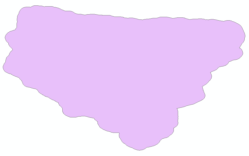
The goal of this project is to determine if a similar trend of narrowing Bankfull Width in the headwater reaches, and slight widening in the downstream reaches of watersheds has continued in Southwestern Wisconsin, Specifically in the Western Ames Fork of the Pecatonica River Watershed (Figure 1). In the mid 1930s the SCS soil conservation services implemented improved agricultural practices in an effort to protect the land and try to revert land back to presettlement times where streams were healthy in Wisconsin. I previously did similar research in the Galena River watershed (Figure 2), where data from 2017 was compared to data found in literature that compared linear regression lines from 1940 to 1979. In 2017 myself and a few other students from Missouri State performed field work in the Galena Watershed, where lead and zinc was being traced through sediment samples. Additionally to collecting soil samples, Bankfull Width was determined at each site. This measurement was the basis for my study. Bankfull width will again be utilized, however measurements were collected through imagery rather than field work. 

Figure 1:Study Area for Western Ames Branch

Figure 2:Galena River Map

Outline of Goals

Digitize study area

Digitize sample locations

Clip raster imagery to study area

Delineate watershed in study area

Delineate streams

Digitize drainage areas at each sample site

Measure bankfull width at each sample site

Create a linear regression to compare to data from literature

Literature Review

Frank Magilligan (1985) conducted a study where he compared data from the soil conservation services (SCS) to his own data in 1979. Both sets of data compared bankfull width to drainage area (Figure 3). Magilligan noted in his work that upper reaches of the watershed became narrower in 1979 than in 1940. Knox (1977) noted that larger more frequent floods occurred in the upper reaches of watersheds, and he attributed this to poor agricultural practices. Gebert and Krug (1996) noted that magnitude and frequency of floods throughout the watershed system have decreased, and they attribute this to improved agricultural and land use practices such as contour farming (Figure 4) and strip cropping.

Figure 3: Frank Magilligans Linear Regression coparison.

Figure 4: Contour strip farming, an improved agricultural practice.

Data
In the digitizing process three data sources were used, Lafeyette county Wisconsin LiDar with an underlying Topographic Basemap, (Figure 5) and a 30 arc second DEM of North America (Figure 6).

Figure 5: Lidar DEM overlayed on a topographic basemap, this allowed for ease in digitizing, when determining drainage divides in the topography of the study area.

Figure 6: Map showing the 30 arc-second DEM of North America.

Methods
Digitization, and statistical analysis

Numerous steps were taken in completing this project. First The study area was digitized, this was done by arbitrarily choosing a branch of a watershed nearby where my previous research was done by the Galena watershed. To determine the study area I choose the Ames western branch, and digitized around the highest elevation, which created a polygon around a small portion of the Watershed (Figure 7). Then sample locations were placed along streams within the study area (Figure 8). These locations were chosen in areas, where there is a visible bank, and these locations tend to be seen before or after a bend in a stream. in order to gather my bankfull data, i needed to utilize the measure tool and high resolution imagery, to measure the streams (Figure 9), once these numbers were gathered they were entered into an excel table, where drainage area will soon become a part. Next each drainage area above each sample site was digitized using the same method as in digitizing the study area, where the highest elevation around a drainage area is used when digitizing (Figure 10). once these individual polygons are created, it is necessary to merge all polygons above one sample location to determine an accurate drainage area. this means at the lowest point on the river, that points drainage area consists of every single polygon up stream (Figure 11) (Figure 12). Next the drainage area of each polygon was associated in an excel table with its respective bankfull width, and a regression analysis was performed.

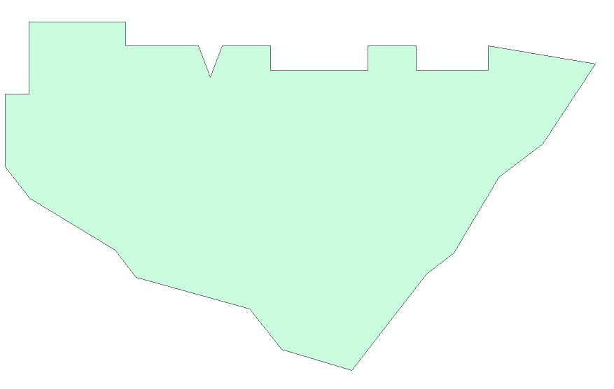
Figure 7: Digitized study area

Figure 8: Sample locations

Figure 9: measuring process used for determining Bankfull Width.

Figure 10: Each drainage area above each sample location is digitized.

Figure 11: All polygons layered on top of each other after being merged.

Figure 12: Sample site 19 is shown in green, and encompasses the entire extent of the study area because it is at the lowest point in the watershed. Sample site 15 starts halfway through the study area but encompasses the entire area above its location, and also the area under sample site 5.

Watershed and Stream Delineation

In this next section, a stream delineation and watershed delineation was performed through the use of Model maker, and numerous different tools (Figure 13). First the study area (Figure 14) was buffered by .5 kilometers (Figure 15), to allow the watershed delineation to be more accurate. Then the DEM was clipped to the buffered study area (Figure 16), then a fill was performed to get rid of sinks within the image (Figure 17). Next a Flow Direction raster was created (Figure 18), followed by Flow Accumulation (Figure 19), a conditional argument (Figure 20), Stream order (Figure 21), stream to feature (Figure 22), basin (Figure 23), and finally raster to polygon (Figure 24).

Figure 13: Full model

Figure 14: Study_Area

Figure 15: Study_Area_Buffer1

Figure 16: DEM_Buffer_Clip

Figure 17: Fill

Figure 18: Flow_Dir

Figure 19: Flow_Accumulation

Figure 20: Net_50k

Figure 21: Stream_order

Figure 22: streamfeatures

Figure 23: Basin

Figure 24: Basin_poly

Results
A bankfull width to drainage area linear regression was created (Figure 25). The results of the comparison were hopefully going to show a positive linear slope, this would mean that my hypothesis of improved agricultural practices is shaping the streams and reverting them back to a similar state as presettlement streams prior to people living in Wisconsin. However this was not the case, and i believe it is due to performing the study over too small of a portion of the watershed. 

The stream and watershed delineation produced two outputs shown above in FIgures 22 and 24. these were used as a visible comparison to see if my digitized area was similar to what the GIS could produce through a model.

Figure 25: Linear regression between bankfull width and drainage area.

Sources

Gebert, W.A., and Krug, W.R. 1996. Streamflow trends in Wisconsin’s Driftless Area. Journal of the American Water Resources Association 32: 733-744.

Knox, J.C. 1977. Human impacts on Wisconsin stream channels. Annals of the Association of American Geographers 67: 323-342.

Magilligan, F.J. 1985. Historical floodplain sedimentation in the Galena River Basin, Wisconsin and Illinois. Annals of the Association of American Geographers 75: 583-594

DEM Source

National Aeronautics and Space Administration (NASA), the United Nations Environment Programme/Global Resource Information Database (UNEP/GRID), the U.S. Agency for International Development (USAID), the Instituto Nacional de Estadistica Geografica e Informatica (INEGI) of Mexico, the Geographical Survey Institute (GSI) of Japan, Manaaki Whenua LandcareResearch of New Zealand, and the Scientific Committee onAntarctic Research (SCAR).